Mechanical characterization of potato parenchyma under different turgor states

Internship project: Imran - Bio-Inspired Systems team, Institut des Sciences du Mouvement. Study of how osmotic state influences the stiffness and deformation of potato parenchyma.

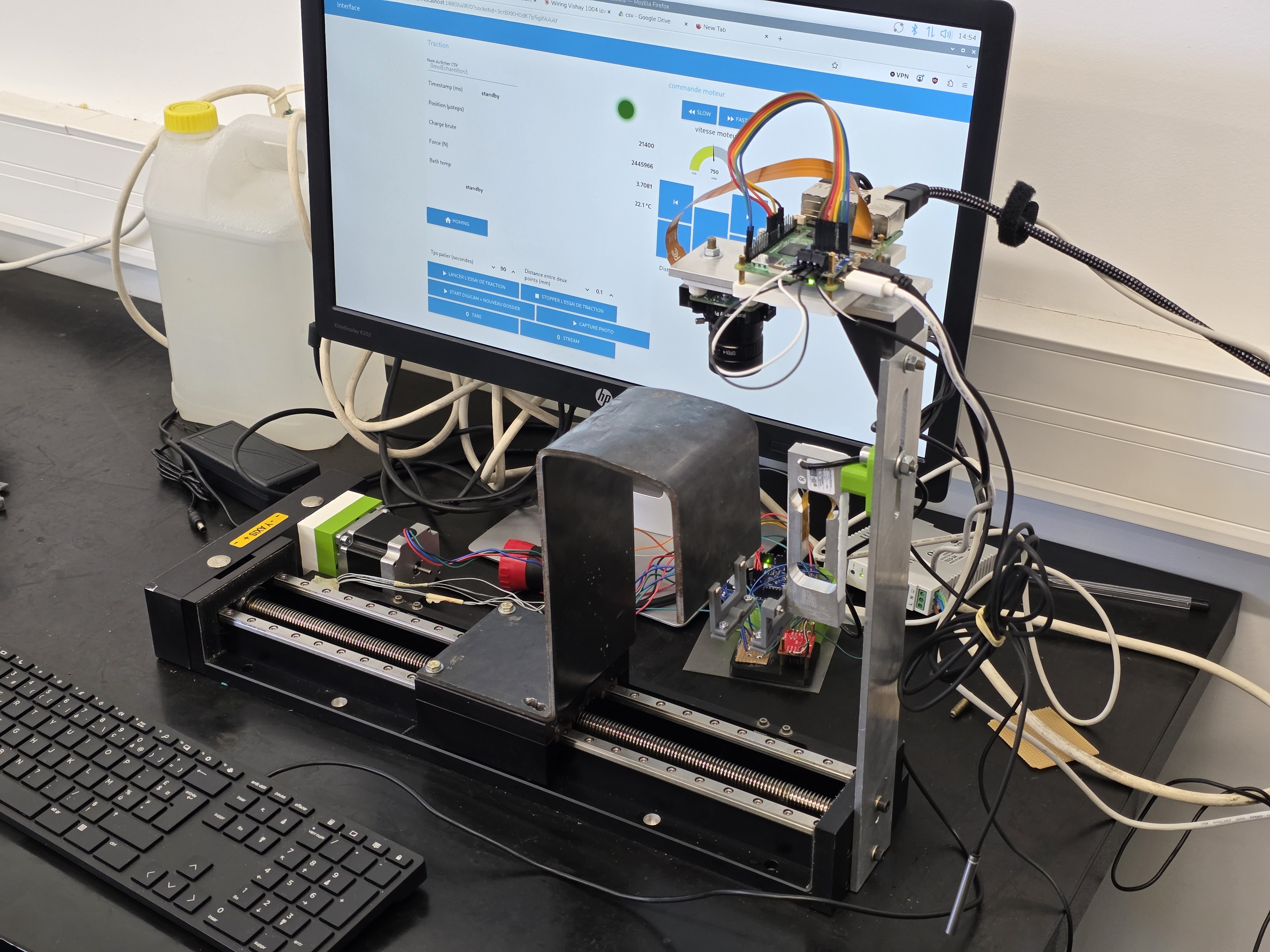
Potato-parenchyma traction bench used for mechanical characterization.
Internship project: Imran
Supervisor: Loïc TADRIST
Team: Bio-Inspired Systems (SBI)
Laboratory: Institut des Sciences du Mouvement (ISM)
Topics: plant biomechanics, turgor pressure, tensile testing and bio-inspired instrumentation

How does the pressure inside plant cells influence tissue stiffness?

This project studies the mechanical behavior of potato parenchyma when its turgor state changes. Samples are placed in different sorbitol solutions and then tested with an instrumented traction bench.

1. Scientific context

The Bio-Inspired Systems team studies how plants generate motion, resist mechanical loads and adapt their structure to their environment. Potato parenchyma is a useful model tissue because its mechanical behavior depends strongly on water content and turgor pressure.

2. Objective of the internship

The objective is to characterize the mechanical response of potato parenchyma under different osmotic conditions. Sorbitol solutions are used to modify the water balance of the samples, then tensile tests are performed to compare stiffness, deformation and apparent Young modulus.

3. Sample preparation

The samples are cut from potato parenchyma and prepared as small test specimens. Their geometry must be controlled because the measured mechanical properties depend on the useful length, diameter and gripping conditions.

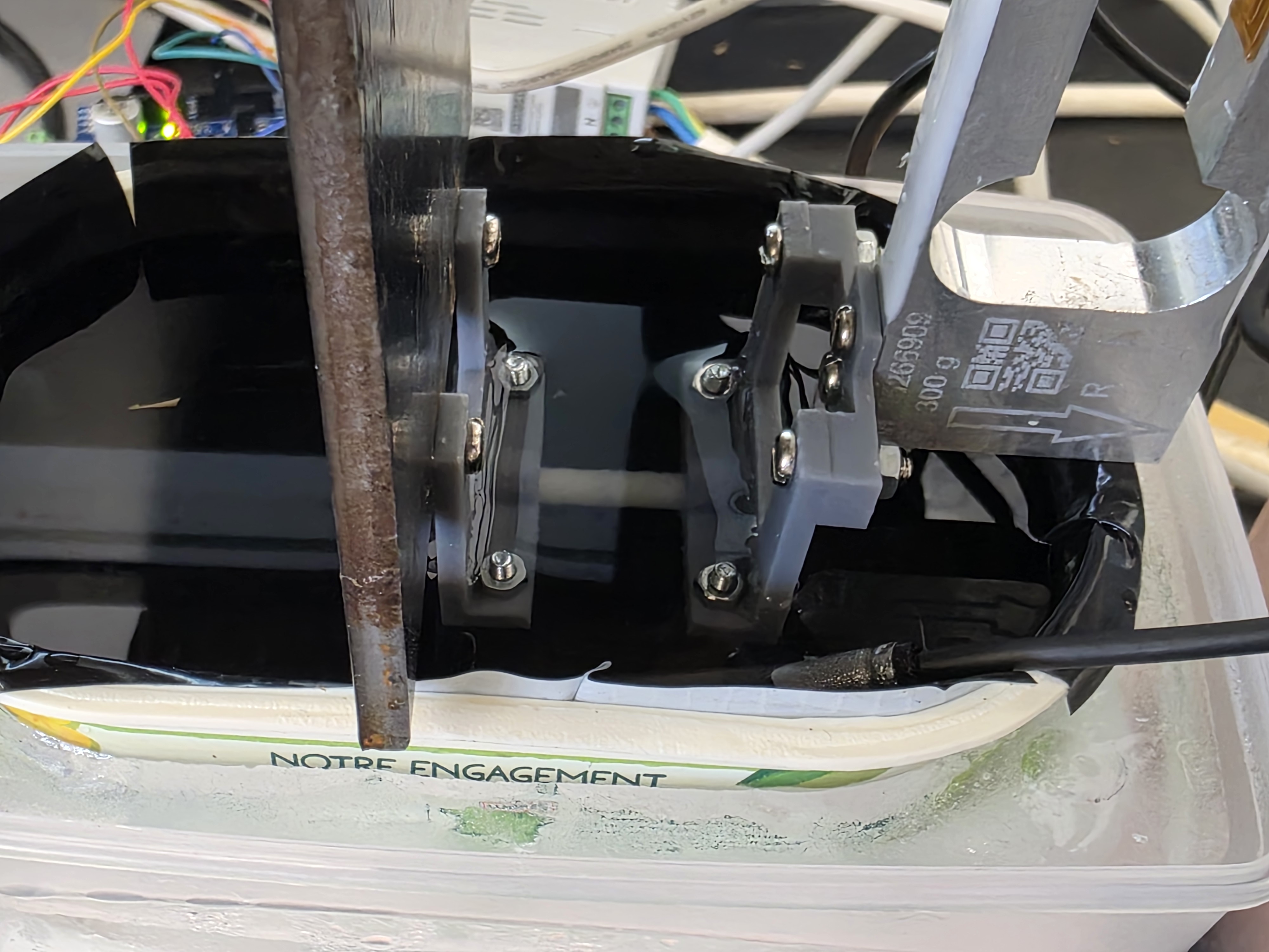
Sample installed on the traction bench

Potato sample mounted between the grips of the traction bench.

Potato-parenchyma sample held between the grips of the traction bench before a tensile test.

4. Instrumented traction bench

The experiments are performed on a custom traction bench. A motor applies a controlled displacement while sensors record force and displacement. The bench also includes optical acquisition to follow the deformation of the sample.

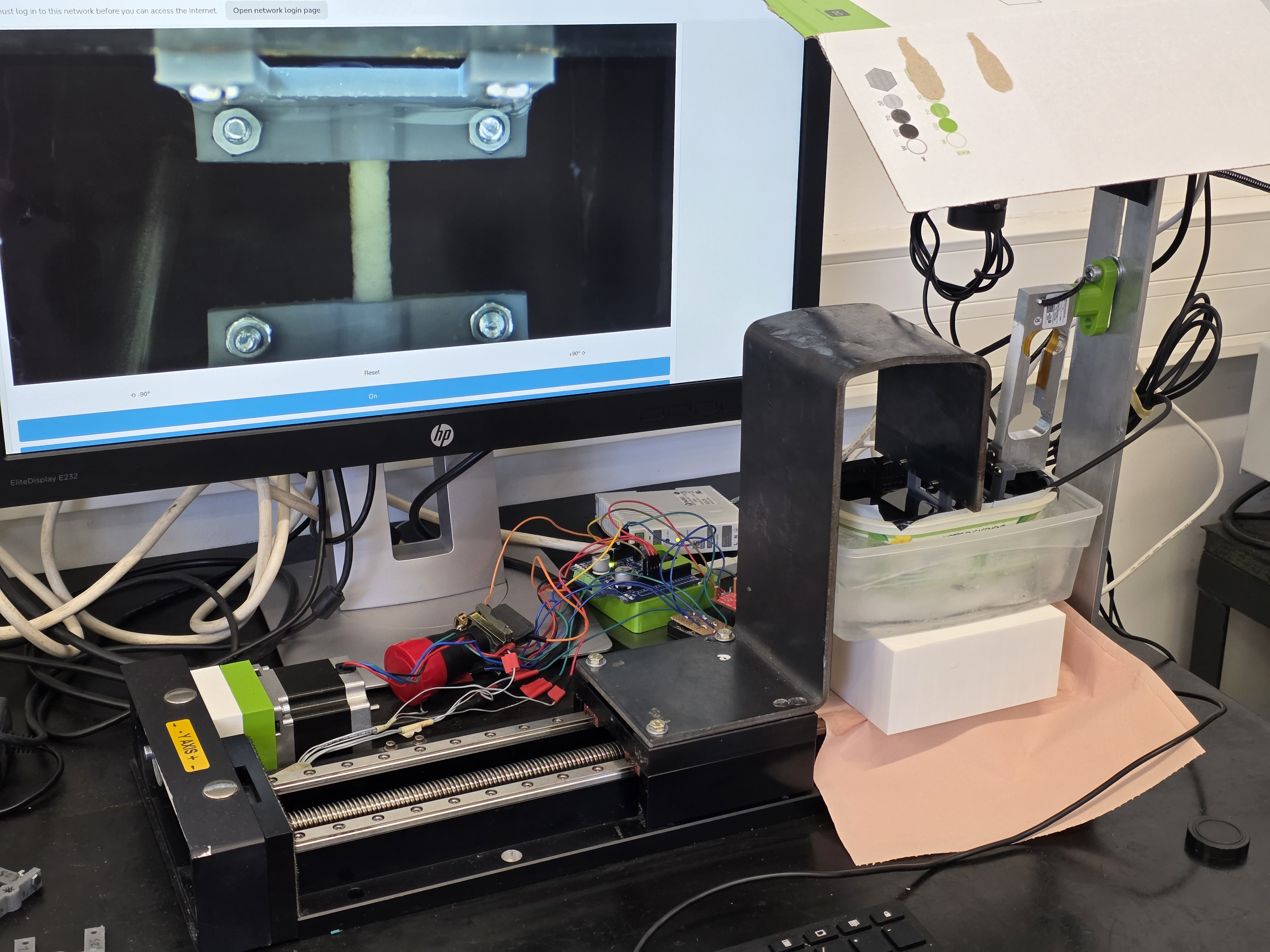
Traction bench during operation

Instrumented traction bench operating with a potato-parenchyma sample.

The camera makes it possible to observe the sample during traction and synchronize image analysis with mechanical measurements.

5. Optical acquisition and instrumentation

A high-resolution camera connected to a Raspberry Pi 5 follows the deformation of the sample. The Raspberry Pi also centralizes data acquisition and communicates with the control electronics.

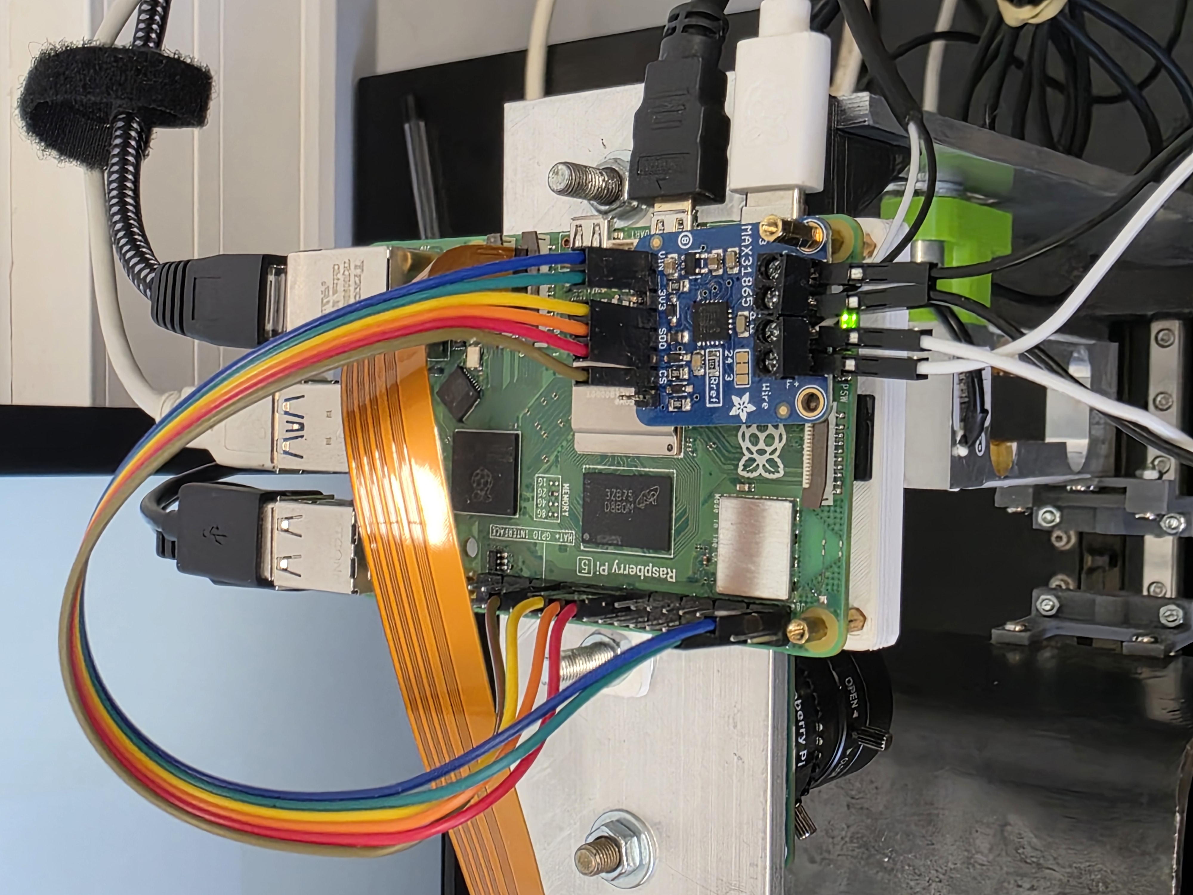
Raspberry Pi and acquisition modules

Raspberry Pi 5 and electronic acquisition modules.

The Raspberry Pi 5 centralizes the control of the bench and the acquisition of several measurement channels.

6. Data processing

The data-processing workflow combines mechanical measurements and image analysis. MATLAB scripts convert the raw files, detect useful loading steps, estimate Young modulus and compare the results across concentrations.

7. Node-RED acquisition

The experimental acquisition is driven with Node-RED on a Raspberry Pi 5. The workflow controls the Arduino, the stepper motor, the load cell and synchronized image capture.

MATLAB code: Data_treatment.m

Main data-processing script. It converts raw CSV measurements, detects loading steps and estimates the apparent Young modulus from force-displacement data.

Data_treatment.m matlab
clearclose allclc % =====================================================================%  Data_treatment - corrected June 2026%%  Changes vs Data_treatment_2025_10_16.m:%   (1) FORCE: was `Data(:,4)*10` (no calibration at all). Now uses the%       new load cell's factor. New cell (June 2026): 0.00015443 g/count.%       force_mN = raw * 0.00015443 g/count * 9.81 mN/g = raw * 1.5150e-3%       Le compte brut devient POSITIF en traction sur cette cellule :%       pas de signe moins (tirer -> force positive).%       Sign: tensile produces NEGATIVE raw counts, so the minus makes%       tension come out positive.%   (2) POSITION: was `/1600*2` (= 800 steps/mm) - WRONG for this bench.%       The bench is 2510 µsteps/mm in 1/32 microstepping. Using 800%       under-counted displacement by ~3.14x and would have made E ~3x%       too large. Now divides by 2510.%   (3) ENCODER: column 3 is no longer populated (no encoder on this%       bench - the Arduino always emits 0 there). The old encoder plots%       used xlim/ylim([min max]) on an all-zero vector, which throws an%       error and halts the script before the analysis runs. Those plots%       are removed. The modulus analysis never used the encoder anyway.%%  Palier-averaging logic and the .mat save are unchanged.% ===================================================================== concentration = "0.5";mass_sorbitol = "36.43g"; % --- Calibration constants -------------------------------------------FORCE_MN_PER_RAW = 1.5150e-3;    % mN per raw count. NB: raw count goes POSITIVE                                 % under tension on this cell, so NO minus sign                                 % (pulling -> positive force).USTEPS_PER_MM    = 2510;         % 1/32 microstepping, measured at the bench % base_folder = 'G:\Traction parenchyme pomme de terre\BANC_TOLE';base_folder = 'C:\Users\imran\OneDrive\Documents\MATLAB\potato\0,5mol';folder_name = '0,5molEchantillon5\';path = [base_folder '\RAW_DATA\' folder_name];directoryContent = dir(path); for i=1 : length(directoryContent)    disp(directoryContent(i).name)    if contains(directoryContent(i).name, '.csv')        csv_name = directoryContent(i).name;    endend % --- lecture ROBUSTE du CSV ------------------------------------------%  Tolere : (a) un en-tete present ou absent, (b) des lignes parasites%  AVANT le vrai en-tete (banc au repos avant le demarrage de l'essai,%  qui re-ecrit l'en-tete). On detecte la DERNIERE ligne "Timestamp(ms)"%  et on lit a partir de la ; sinon on lit tout en numerique.fid = fopen([path csv_name]); raw_lines = textscan(fid,'%s','Delimiter','\n','Whitespace',''); fclose(fid);raw_lines = raw_lines{1};hdr_idx = find(contains(raw_lines,'Timestamp(ms)'), 1, 'last');   % derniere occurrenceif isempty(hdr_idx)    Data = readmatrix([path csv_name]);                          % pas d'en-tete : tout numeriqueelse    Data = readmatrix([path csv_name], 'NumHeaderLines', hdr_idx); % saute en-tete + parasitesendData = Data(all(~isnan(Data(:,1:2)),2), :);   % vire d'eventuelles lignes vides/NaN % CSV columns: 1 = timestamp(ms), 2 = motor position(µsteps),%              3 = unused (always 0, no encoder), 4 = raw HX711 counttime = (Data(:,1)-Data(1,1))/1000 ;                       % sforce = Data(:,4) * FORCE_MN_PER_RAW;                     % mNdisplacement_moteur = (Data(:,2)-Data(1,2)) / USTEPS_PER_MM;  % mm % NOTE ON SIGN: the essai now pulls in the +1 (FWD) direction, so motor% position increases during the pull and displacement_moteur is positive.% If you ever see it come out negative (force-displacement curve in the% wrong quadrant, or 0 paliers detected below), the pull direction was% reversed - just put a leading minus back on the line above. figure;subplot(3,1,1)plot(time, force);xlabel('time (s)'); ylabel('force (mN)');subplot(3,1,2)plot(time, displacement_moteur)xlabel('time (s)'); ylabel('displacement moteur (mm)');subplot(3,1,3)plot(displacement_moteur, force)xlabel('displacement moteur (mm)'); ylabel('force (mN)'); % --- Palier detection (unchanged) ------------------------------------dev= (diff(displacement_moteur)./ diff(time)) > (0.1/1); % 0.1mm en 1 secddev= diff(dev);paliers=zeros(1, length(time));paliers(1)=0;for i=1:length(ddev)    if ddev(i)>0        paliers(i+1) = paliers(i)+1;    else        paliers(i+1) = paliers(i);    end endpaliers(end)=paliers(end-1); for i=1:max(paliers)    force_palier = force(paliers==i);    displacement_palier = displacement_moteur(paliers==i);    force_palier= force_palier (floor(length(force_palier)/2):end);    displacement_palier = displacement_palier(floor(length(force_palier)/2):end);    MeanForce(i)= mean(force_palier);    Mean_disp(i)= mean(displacement_palier);    TempsPalier(i) = mean(time(paliers==i));end figure;plot(Mean_disp, MeanForce, '+r')xlabel('Mean\_disp (mm)')ylabel('MeanForce (mN)') %% =====================================================================%  MODULE DE YOUNG  E = sigma / epsilon%  E = (pente force-deplacement) * L0 / A%  Force en mN, deplacement et L0 en mm, A en mm^2  ->  E en kPa%  (1 mN/mm^2 = 1 kPa)%  -> EDITER L0 et d pour CHAQUE essai.% =====================================================================L0 = 16.94;           % longueur utile = BLANC EXPOSE entre mors, mm (pied a coulisse)                     %   (PAS les 30.98 mm mors-a-mors : la partie serree ne se deforme pas)d  = 4.33;           % diametre echantillon GONFLE (apres trempage), mm                     %   ~4.92 mesure sur l'image ; coherent avec 4.85-5.1 au pied a coulisse.                     %   -> coherent avec le diametre mesure au pied a coulisse.A  = pi*(d/2)^2;     % section, mm^2  (cylindre) % Region lineaire utilisee pour la pente : indices des paliers.% Par defaut la 1ere moitie. REGARDER la figure et ajuster si besoin,% p.ex.  idx = 1:15;  pour ne garder que le debut rectiligne.idx = 1:round(numel(Mean_disp)/2); pfit  = polyfit(Mean_disp(idx), MeanForce(idx), 1);slope = pfit(1);                 % mN/mmE_kPa = slope * L0 / A;          % kPa % droite ajustee superposee sur la courbehold onplot(Mean_disp(idx), polyval(pfit, Mean_disp(idx)), '-k', 'LineWidth', 1.5)hold offtitle(sprintf('pente = %.2f mN/mm   ->   E = %.1f kPa  (%.3f MPa)', ...              slope, E_kPa, E_kPa/1000)) fprintf('\n=== Module de Young ===\n');fprintf('L0 = %.2f mm | d = %.2f mm | A = %.2f mm^2\n', L0, d, A);fprintf('points utilises (lineaire) : %d a %d sur %d paliers\n', ...        idx(1), idx(end), numel(Mean_disp));fprintf('pente = %.3f mN/mm\n', slope);fprintf('E = %.1f kPa  (= %.4f MPa)\n', E_kPa, E_kPa/1000); %% =====================================================================%  COURBE CONTRAINTE-DEFORMATION  (sigma vs epsilon)  -- graphe pour M. Tadrist%  sigma = Force / A0   (MPa) ;  epsilon = deplacement / L0  (sans unite)%  NB : epsilon ici = deformation MOTEUR (crosshead). Le glissement aux%  mors la surestime ; E corrige reel = via Verif_manuelle_multi (clics).% =====================================================================epsilon  = Mean_disp / L0;                 % deformation (motor/crosshead)sigma    = (MeanForce/1000) / A;           % MPa  (mN->N, /mm^2) pE   = polyfit(epsilon(idx), sigma(idx), 1);Emod = pE(1);                              % MPa = pente sigma/epsilon figure;plot(epsilon, sigma, '+r'); hold on;plot(epsilon(idx), polyval(pE, epsilon(idx)), '-k', 'LineWidth', 1.5); hold off;xlabel('\epsilon  (deformation)'); ylabel('\sigma  (MPa)');title(sprintf('Contrainte-deformation 0 mol/L   |   E = %.3f MPa (apparent, moteur)', Emod));grid on; fprintf('\n=== Courbe sigma-epsilon ===\n');fprintf('E (pente sigma/epsilon, deformation moteur) = %.3f MPa\n', Emod);fprintf('   -> APPARENT (course moteur). E corrige = via Verif_manuelle_multi (clics).\n'); %% =====================================================================%  SAUVEGARDE (E APPARENT seulement)%  Le E corrige du glissement n'est PLUS calcule ici : il provient%  desormais du pointage MANUEL des points (Verif_manuelle_multi.m),%  bien plus fiable que l'ancienne detection automatique d'images.%  -> Ce script ne fait qu'une chose : le E APPARENT (force vs moteur).% =====================================================================save([base_folder '\META_DATA_TOLE\' folder_name 'force_temps.mat'], ...    "Mean_disp", "MeanForce", "time", "TempsPalier", "force", ...    "concentration", "mass_sorbitol", ...    "L0", "d", "A", "slope", "E_kPa", '-mat') 

MATLAB code: Image_treatment_dots.m

Image-processing script used to detect marking dots, follow their displacement and estimate lateral deformation during traction tests.

Image_treatment_dots.m matlab
clear; close all; clc; % =====================================================================%  Image_treatment_dots.m   v7  (white sample, TWO dark dots)%%  Suit la DISTANCE entre deux points marques sur la jauge -> allongement%  REEL du materiau (insensible au glissement). H_mm = distance points,%  D_mm = diametre a mi-distance, nu = -eps_lat/eps_axial.%  Sauvegarde le MEME .mat que les autres scripts image.%%  -----------------------------------------------------------------%  CHANGEMENT v6 -> v7 (corrige la detection sur images SOMBRES) :%   v6 : seuil FIXE (dot_dark_frac * luminosite). Sur images peu eclairees%        les points gris passaient sous le bruit -> 0/6/1 points detectes,%        distance erratique, allongement parfois NEGATIF (E corrige absurde).%   v7 : seuil ADAPTATIF par image. On isole d'abord la colonne, puis on%        prend les pixels les plus SOMBRES de l'interieur (percentile bas)%        comme candidats-points, on enleve le bruit (ouverture morpho), et%        on garde les 2 plus GROS blobs proches de l'axe. Beaucoup plus%        robuste a un eclairage faible/variable.%        -> verifie sur 0,1molEchantillon2 : 60/61 images, distance%           croissante et monotone.%%  Necessite l'Image Processing Toolbox (bwconncomp/regionprops/imopen).%  A EDITER : base_folder, folder_name, scale ; au besoin dot_pct.% ===================================================================== base_folder = 'C:\Users\imran\OneDrive\Documents\MATLAB\potato\0,2mol';folder_name = '0,2molEchantillon2\';scale = 0.02239;          % mm/pixel -- re-deriver si distance/zoom change band_frac   = 0.075;      % demi-largeur bande centrale (fraction largeur image)row_lo = 0.40; row_hi = 0.88;min_contrast = 25;edge_margin  = 0.20;      % fraction de largeur ignoree de chaque bord (evite le fond)dot_pct      = 2.5;       % les pixels < ce percentile (interieur) = candidats-points                          %   (monter a ~4 si points peu visibles ; baisser si trop de bruit)dot_min_area = 8;         % aire mini d'un point (px)dot_max_area = 2500;      % aire maxi (px) -- rejette grosse ombreaxis_tol     = 0.35;      % un point doit etre a < axis_tol*largeur_bande de l'axemin_sep_frac = 0.30;      % les 2 points separes de > min_sep_frac * hauteur jaugedebug_first  = true;      % entoure les points sur la 1ere image (VERIFIER) % ---------------------------------------------------------------------path  = [base_folder '\RAW_DATA\' folder_name];files = dir([path '*.jpg']);if isempty(files), error('Aucune image .jpg dans %s', path); end[~,order] = sort({files.name}); files = files(order);n = numel(files); t = nan(n,1); H_mm = nan(n,1); D_mm = nan(n,1);xc_anchor = []; for k = 1:n    name = files(k).name;    I = imread([path name]);    if size(I,3)==3, G = double(rgb2gray(I)); else, G = double(I); end    [Himg,Wimg] = size(G);    xc = round(Wimg/2); dx = round(Wimg*band_frac);    x0 = max(1,xc-dx);    band = G(:, x0:min(Wimg,xc+dx));    bw_px = size(band,2);    if isempty(xc_anchor), xc_anchor = bw_px/2; end     r0s = max(1, round(row_lo*Himg));    r1s = min(Himg, round(row_hi*Himg));     % --- 1) colonne SAMPLE : bords par ligne, suite continue ---    yj=[];L=[];R=[];cs=[];    for r = r0s:r1s        prof = band(r,:); pk = max(prof); bg = prctile(prof,20);        if pk-bg < min_contrast, continue; end        half = 0.5*(pk+bg); above = prof>half;        if ~any(above), continue; end        dd=diff([false,above,false]); st=find(dd==1); en=find(dd==-1)-1; ctr=(st+en)/2;        [dist,wi]=min(abs(ctr-xc_anchor));        if dist>0.5*bw_px || en(wi)<=st(wi), continue; end        yj(end+1)=r; L(end+1)=st(wi); R(end+1)=en(wi); cs(end+1)=ctr(wi); %#ok<AGROW>    end    if numel(yj)<30, warning('%s : echantillon non trouve', name); continue; end    yj=yj(:);L=L(:);R=R(:);cs=cs(:);    sp=find(diff(yj)>5); ss=[1;sp+1]; ee=[sp;numel(yj)];    [~,bi]=max(ee-ss); ix=ss(bi):ee(bi);    yj=yj(ix);L=L(ix);R=R(ix);cs=cs(ix);    top=yj(1); bot=yj(end); gauge_h=bot-top;    xc_anchor = median(cs);     % --- 2) interieur du sample + valeurs ---    interior = false(size(band)); vals=[];    for j=1:numel(yj)        w=R(j)-L(j); m=round(edge_margin*w); a=L(j)+m; b=R(j)-m;        if b>a, interior(yj(j),a:b)=true; vals(end+1:end+(b-a+1))=band(yj(j),a:b); end %#ok<AGROW>    end    if numel(vals)<50, continue; end     % --- 3) POINTS = pixels les plus sombres (seuil ADAPTATIF par percentile) ---    thr = prctile(vals, dot_pct);    BWdot = (band <= thr) & interior;    BWdot = imopen(BWdot, strel('disk',1));          % enleve le bruit 1px    CC = bwconncomp(BWdot); rp = regionprops(CC,'Centroid','Area');    cents=[]; areas=[];    for i=1:numel(rp)        if rp(i).Area<dot_min_area || rp(i).Area>dot_max_area, continue; end        if abs(rp(i).Centroid(1)-xc_anchor) > axis_tol*bw_px, continue; end        cents=[cents; rp(i).Centroid]; areas=[areas; rp(i).Area]; %#ok<AGROW>    end    if size(cents,1)<2        warning('%s : moins de 2 points (monter dot_pct ?)', name); continue;    end     % garder les 2 plus GROS (vrais points > mouchetures), puis ordonner par y    [~,is]=sort(areas,'descend');    keep=cents(is(1:min(3,numel(is))),:);    [~,iy]=sort(keep(:,2));    cTop=keep(iy(1),:); cBot=keep(iy(end),:);    dot_dist = hypot(cBot(1)-cTop(1), cBot(2)-cTop(2));    if dot_dist < min_sep_frac*gauge_h        warning('%s : 2 points trop proches (%.0f px) -> ignore', name, dot_dist); continue;    end     % --- diametre sous-pixel a mi-distance ---    ymid = min(max(round(mean([cTop(2) cBot(2)])), top), bot);    prof = band(ymid,:); pk=max(prof); bg=prctile(prof,20); half=0.5*(pk+bg);    above=prof>half; dd=diff([false,above,false]); st=find(dd==1); en=find(dd==-1)-1;    ctr=(st+en)/2; [~,wi]=min(abs(ctr-xc_anchor)); l=st(wi); rr=en(wi);    if l>1,            xl=l-1+(half-prof(l-1))/(prof(l)-prof(l-1)+1e-9); else, xl=l; end    if rr<numel(prof), xr=rr+(half-prof(rr))/(prof(rr+1)-prof(rr)-1e-9); else, xr=rr; end    width_px = xr-xl;     t(k)    = str2double(name(1:2))*3600 + str2double(name(3:4))*60 + str2double(name(5:6));    H_mm(k) = dot_dist * scale;    D_mm(k) = width_px * scale;     if debug_first        figure('Name','VERIF points (1ere image)');        imshow(uint8(band)); hold on;        plot(cTop(1),cTop(2),'go','MarkerSize',16,'LineWidth',2);        plot(cBot(1),cBot(2),'go','MarkerSize',16,'LineWidth',2);        plot([cTop(1) cBot(1)],[cTop(2) cBot(2)],'g-');        plot([xl xr],[ymid ymid],'c-','LineWidth',2);        title('VERIFIER : 2 cercles verts = vos points ; cyan = diametre');        hold off; debug_first=false;    endend ok = ~isnan(t); t=t(ok); H_mm=H_mm(ok); D_mm=D_mm(ok);if numel(t)<3, error('Trop peu de frames exploitables (%d).', numel(t)); endt = t - t(1); eps_axial = (H_mm - H_mm(1)) / H_mm(1);eps_lat   = (D_mm - D_mm(1)) / D_mm(1);pN = polyfit(eps_axial, eps_lat, 1); nu = -pN(1); figure;subplot(2,1,1); plot(t,H_mm,'-o'); grid on;xlabel('temps (s)'); ylabel('distance points (mm)'); title('Allongement reel (entre points)');subplot(2,1,2); plot(t,D_mm,'-o'); grid on;xlabel('temps (s)'); ylabel('diametre (mm)'); title('Diametre sous-pixel'); figure;plot(eps_axial, eps_lat, '+r'); hold on;plot(eps_axial, polyval(pN,eps_axial), '-k','LineWidth',1.5); hold off; grid on;xlabel('\epsilon_{axial} (points)'); ylabel('\epsilon_{lateral}');title(sprintf('Poisson  \\nu = %.3f', nu)); fprintf('\n=== Image (suivi de points, v7) ===\n');fprintf('frames exploitees = %d / %d\n', numel(t), n);fprintf('distance initiale points = %.2f mm | diametre initial = %.2f mm\n', H_mm(1), D_mm(1));fprintf('allongement reel final = %.2f mm -> deformation axiale = %.3f\n', H_mm(end)-H_mm(1), eps_axial(end));fprintf('variation diametre = %+.1f %% | nu = %.3f\n', (D_mm(end)/D_mm(1)-1)*100, nu); if D_mm(end) >= D_mm(1)    warning('Diametre non decroissant -> Poisson NON FIABLE.');elseif nu<0 || nu>0.5    warning('nu=%.3f hors [0;0.5] -> a verifier.', nu);else    fprintf('-> diametre decroissant et nu dans [0;0.5] : POISSON PLAUSIBLE.\n');endif any(diff(H_mm) < -0.05*H_mm(1))    warning('Distance points non monotone -> un point a saute, verifier la detection.');else    fprintf('-> distance points monotone : allongement/glissement FIABLE.\n');end save([base_folder '/META_DATA_TOLE/' folder_name 'width_temps.mat'], ...     't','H_mm','D_mm','eps_axial','eps_lat','nu','scale','-mat'); 
MATLAB code: Plot_E_vs_concentration.m

Summary script used to compare the Young modulus with sorbitol concentration and visualize the experimental results.

Plot_E_vs_concentration.m matlab
clear; close all; clc;% =====================================================================%  Plot_E_vs_concentration.m%%  Courbe E (apparent ET corrige) en fonction de la concentration.%   - E apparent : lu dans chaque force_temps.mat (Data_treatment)%   - E corrige  : lu dans RESULTATS_manuel.xlsx (pointage MANUEL,%                  Verif_manuelle_multi) -- SOURCE UNIQUE du corrige.%%  Graphe AGREGE -> sauvegarde a la RACINE (root).% ===================================================================== root = 'C:\Users\imran\OneDrive\Documents\MATLAB\potato\';xlsx = [root 'RESULTATS_manuel.xlsx']; % --- exclusions (nom d'echantillon EXACT) ----------------------------exclude_app  = {'0,4molEchantillon1'};exclude_corr = {'0,2molEchantillon4'};      % corrige aberrant (perte 95%) % --- 1) E APPARENT depuis les force_temps.mat ------------------------conc_dirs = dir([root '*mol']);  conc_dirs = conc_dirs([conc_dirs.isdir]);app = struct('name',{},'conc',{},'Eapp',{});for k = 1:numel(conc_dirs)    cdir = [root conc_dirs(k).name '\META_DATA_TOLE\'];    subs = dir(cdir); subs = subs([subs.isdir] & ~startsWith({subs.name},'.'));    for j = 1:numel(subs)        mf = [cdir subs(j).name '\force_temps.mat'];        if ~isfile(mf), continue; end        S = load(mf); nm = subs(j).name;        if any(strcmp(nm, exclude_app)), continue; end        c = str2double(strrep(strrep(regexprep(nm,'Echantillon.*',''),'mol',''),',','.'));        app(end+1) = struct('name',nm,'conc',c,'Eapp',S.E_kPa/1000); %#ok<SAGROW>    endendif isempty(app), error('Aucun force_temps.mat trouve sous %s', root); end % --- 2) E CORRIGE depuis RESULTATS_manuel.xlsx -----------------------T = readtable(xlsx,'TextType','string');ec = T.E_corr_manuel_MPa;  ec(ec<=0) = NaN;       % garde-fou physiquefor i=1:numel(exclude_corr), ec(T.echantillon==string(exclude_corr{i})) = NaN; end % --- 3) moyennes par concentration -----------------------------------ac = [app.conc]; ae = [app.Eapp]; cc = double(T.concentration_molL);concs = unique([ac, cc.']);mEapp=nan(size(concs)); sEapp=nan(size(concs));mEcor=nan(size(concs)); sEcor=nan(size(concs));for i=1:numel(concs)    a = ae(ac==concs(i));    if ~isempty(a), mEapp(i)=mean(a); sEapp(i)=std(a); end    e = ec(abs(cc-concs(i))<1e-9); e = e(~isnan(e));    if ~isempty(e), mEcor(i)=mean(e); sEcor(i)=std(e); endend % --- 4) figure -------------------------------------------------------f = figure('Color','w','Position',[100 100 760 520]);yyaxis lefterrorbar(concs, mEapp, sEapp, '-o','LineWidth',1.6);ylabel('E apparent (MPa)'); ylim([0 max(mEapp)*1.4]);yyaxis righterrorbar(concs, mEcor, sEcor, '--s','LineWidth',1.6);ylabel('E corrige manuel (MPa)');xlabel('concentration sorbitol (mol/L)');title('E en fonction de la concentration  (apparent vs corrige manuel)');grid on; xlim([min(concs)-0.05 max(concs)+0.05]);legend({'E apparent (moteur)','E corrige (pointage manuel)'},'Location','best'); fprintf('=== E vs concentration ===\n');for i=1:numel(concs)    fprintf(' c=%.1f : E_app %.3f +/- %.3f | E_corr %.2f +/- %.2f MPa\n', ...        concs(i), mEapp(i), sEapp(i), mEcor(i), sEcor(i));end % --- AGREGE -> racine ---saveas(f, [root 'E_vs_concentration.png']);fprintf('-> sauvegarde : %sE_vs_concentration.png\n', root); 

CAD archive of the traction bench

The CAD archive contains the design files of the experimental traction bench. It keeps the mechanical structure, supports, camera holder, Raspberry Pi housing and gripping parts available for future consultation or modification.

Selected STL parts from the traction bench

A few representative STL parts were extracted from the CAD archive so they can be previewed directly on the page. The full technical archive remains available for download.

Loading 3D preview...
STL file available in the web version of the project.

8. Personal contribution

The project builds on a previous experimental setup and focuses on improving the measurement chain, data-processing workflow and reliability of the mechanical characterization.

9. Expected results and perspectives

The experiments aim to compare stiffness and lateral deformation as a function of sorbitol concentration. The results can help connect tissue hydration, turgor pressure and plant mechanical behavior.

Conclusion

This internship combines plant biomechanics, instrumentation, electronics, acquisition software and image processing to study a biological material with controlled experimental tools.

Download this project page

Use this button to open the print dialog, then choose “Save as PDF”.